Interval library in Python

The Python module implements an algebraically closed interval arithmetic for interval computations, solving interval systems of both linear and nonlinear equations, and visualizing solution sets for interval systems of equations.

For details, see the complete documentation on API.

Links

• Article about the library

• Article about the data fitting

• Patent

• Homepage

• Online documentation

• PyPI package

• A detailed monograph on interval theory

Installation

Ensure you have all the system-wide dependencies installed, then install the module using pip:

pip install intvalpy

Examples

Data Fitting:

Suppose the quantity $y$ of interest is described by a function on the variables $x_1, \ldots, x_m$, and this function is

$$ y = f(x, \beta) $$

where $f$ is a fixed expression depending on the vector of independent variables $x = (x_1, \ldots, x_m)$ and the vector of parameters $\beta = (\beta_1, \ldots, \beta_p)$. We want to find the values of the parameters $\beta_1, \ldots, \beta_p$ that best fit the set of values of $x$ and $y$ obtained from measurements or observations of the functional dependency of interest.

Suppose that $n$ values $y^{(i)}$ of the function on sets of arguments $(x_1^{(i)}, \ldots, x_m^{(i)})$ were obtained by observations, where $i = 1, 2, \ldots, n$ is the observation index. The problem statement implies that the equalities

$$ y^{(i)} = f(x_1^{(i)}, \ldots, x_m^{(i)}, \beta_1, \ldots, \beta_p), \quad i = 1, 2, \ldots, n, $$

should be fulfilled, which form a system of equations in the unknowns $\beta_1, \ldots, \beta_p$. By solving this system, we can find the desired values of the parameters that define the functional dependency. However in practice, this system of equations typically lacks traditional solutions due to data errors resulting from inaccurate measurements and uncontrolled external influences. The error may be due to data aggregation or limited amount of data, etc. In such cases, a generalized solution to the resulting system of equations (like a pseudosolution) is typically sought often using probability-theoretic models of data errors. However, in practice the probability distributions of these errors are rarely known precisely, although some assumptions are usually made regarding their characteristics.

The following outlines an approach to estimating the parameters of a function, which leverages the principles and methods of interval analysis. This approach enables the reconstruction of a function using only information about the maximum possible error in the data, without requiring any knowledge or assumptions about the probability distributions of the errors.

import numpy as np
import pandas as pd
import matplotlib.pyplot as plt
import intvalpy as ip

def noise_distribution(n_samples, intensity=0.7, seed=42):
    np.random.seed(seed)
    # Base noise depends on point position
    base_noise = np.random.normal(0, 0.3 * intensity, n_samples)
    # Impulse outliers (rare but noticeable)
    impulse_mask = np.random.random(n_samples) < 0.1  # 10% of points
    impulse_noise = np.random.normal(0, 2 * intensity, n_samples) * impulse_mask
    # Cluster noise (groups of points with similar bias)
    cluster_noise = np.zeros(n_samples)
    n_clusters = max(2, n_samples // 20)
    cluster_centers = np.random.choice(n_samples, n_clusters, replace=False)
    for center in cluster_centers:
        cluster_size = np.random.randint(2, 6)
        cluster_indices = np.clip(np.arange(center-2, center+3), 0, n_samples-1)
        cluster_value = np.random.normal(0, 1.5 * intensity)
        cluster_noise[cluster_indices] += cluster_value
    # Combine all components
    return base_noise + impulse_noise + 0.4*cluster_noise

# Original function
def f(x): 
    return -5.24 + x*np.sin(x)
    
# Data generation
x = np.sort(np.random.uniform(0.1, 9.9, 100))
y = f(x)
const = np.ones(len(x))
eps_x = noise_distribution(len(x), intensity=0.005, seed=42)
eps_y = noise_distribution(len(x), intensity=1.75, seed=43)
x_noisy = x + eps_x
y_noisy = y + eps_y
df = pd.DataFrame(
    data = np.array([ const, x_noisy, y_noisy ]).T,
    columns = ['const', 'x', 'y']
)
# Convert to interval uncertainty
df['x'] = df['x'] + ip.Interval(-max(eps_x), max(eps_x))
df['y'] = df['y'] + ip.Interval(-max(eps_y), max(eps_y))

# Training a polynomial model
model = ip.ISPAE()
model.fit(
    X_train = df[['const', 'x']],
    y_train = df['y'],
    order = [1, 8],
    x0 = None,
    weight = None,
    objective = 'Uni',
    norm = 'inf',
)

# Testing fitted model
ox = np.linspace(0, 10, 1000)
const = np.ones(len(ox))
df_test = pd.DataFrame(data=np.array([const, ox]).T, columns=['const', 'x'])
y_pred = ip.mid(model.predict(df_test[['const', 'x']]))
y_fact = f(ox)

# Visualization results
fig, ax = plt.subplots(nrows=1, ncols=1, figsize=(10, 3.5))
x_plt = np.array([ip.inf(df['x']), ip.inf(df['x']), ip.sup(df['x']), ip.sup(df['x'])])
y_plt = np.array([ip.inf(df['y']), ip.sup(df['y']), ip.sup(df['y']), ip.inf(df['y'])])
ax.fill(x_plt, y_plt, color='black', alpha=0.15, fill=True, label='Interval uncertainty')
plt.scatter(x_noisy, y_noisy, alpha=0.7, color='black', s=8, label='Noisy data')
plt.plot(ox, y_pred, color='red', ls='--', alpha=1, linewidth=1.5, label='Fitted fucntion')
plt.plot(ox, y_fact, color='black', ls='-', alpha=0.7, linewidth=1.5, label='Original function')
handles, labels = ax.get_legend_handles_labels()
by_label = dict(zip(labels, handles))
ax.legend(by_label.values(), by_label.keys(), loc='lower right')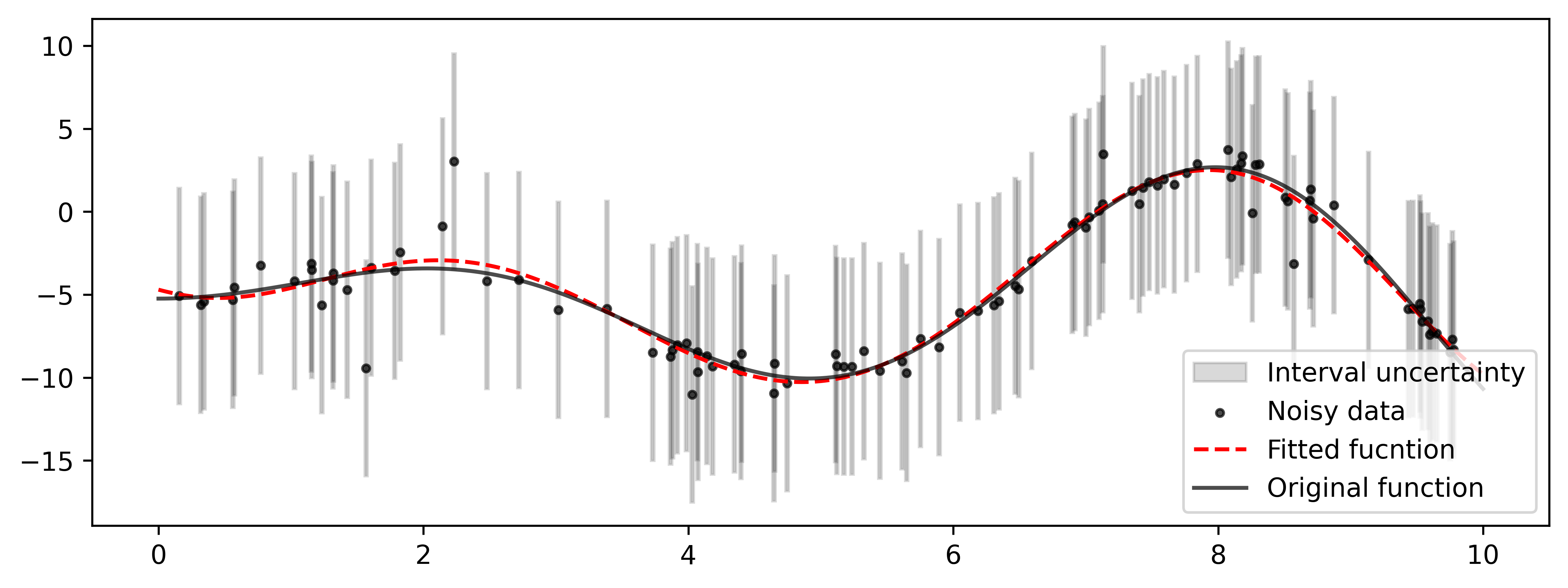

Visualizing solution sets

For a system of linear inequalities of the form A * x >= b or for an interval system of linear algebraic equations A * x = b, the solution sets are known to be polyhedral sets, convex or non-convex. We can visualize them and display all their vertices:

import intvalpy as ip
ip.precision.extendedPrecisionQ = False
import numpy as np


iplt = ip.IPlot(figsize=(15, 15))
fig, ax = iplt.subplots(nrows=2, ncols=2)


#########################################################################
A, b = ip.Shary(2)
shary_uni = ip.IntLinIncR2(A, b, show=False)
shary_tol = ip.IntLinIncR2(A, b, consistency='tol', show=False)

axindex = (0, 0)
ax[axindex].set_title('United and tolerable solution sets for the Shary interval system')
ax[axindex].title.set_size(15)
iplt.IntLinIncR2(shary_uni, color='gray', alpha=0.5, s=0, axindex=axindex)
iplt.IntLinIncR2(shary_tol, color='blue', alpha=0.3, s=10, axindex=axindex)

#########################################################################
A = ip.Interval([
    [[-1, 1], [-1, 1]],
    [[-1, -1], [-1, 1]]
])
b = ip.Interval([[1, 1], [-2, 2]])
unconstrained_set = ip.IntLinIncR2(A, b, show=False)

axindex = (0, 1)
ax[axindex].set_title('Unbounded set')
ax[axindex].title.set_size(15)
iplt.IntLinIncR2(unconstrained_set, color='darkolivegreen', alpha=0.3, s=10, axindex=axindex)

#########################################################################
A = -np.array([[-3, -1],
              [-2, -2],
              [-1, -3],
              [1, -3],
              [2, -2],
              [3, -1],
              [3, 1],
              [2, 2],
              [1, 3],
              [-1, 3],
              [-2, 2],
              [-3, 1]])
b = -np.array([18,16,18,18,16,18,18,16,18,18,16,18])
duodecagon = ip.lineqs(A, b, show=False)

axindex = (1, 0)
ax[axindex].set_title('Duodecagon')
ax[axindex].title.set_size(15)
iplt.lineqs(duodecagon, color='peru', alpha=0.3, s=10, axindex=axindex)

#########################################################################
x = ip.Interval([[1, 1.2], [1.9, 2.7], [1.7, 1.95], [3.5, 3.5],
                 [4.5, 5.5], [6, 6], [6.5, 7.5], [7, 7.8]])
y = ip.Interval([[4, 4.3], [4.5, 5.3], [4.6, 4.8], [5.1, 6],
                 [6, 6.5], [7, 7], [6.7, 7.4], [6.8, 8]])

axindex = (1, 1)
ax[axindex].set_title('Interval scatterplot')
ax[axindex].title.set_size(15)
iplt.scatter(x, y, color='gray', alpha=0.7, s=10, axindex=axindex)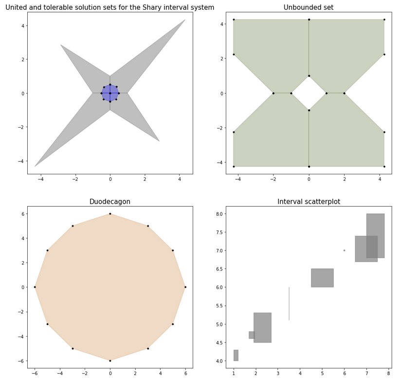

It is also possible to create a three-dimensional (or two-dimensional) slice of an N-dimensional figure to visualize the solution set with fixed N-3 (or N-2) parameters. A specific implementation of this algorithm can be found in the examples.

External decision evaluation:

To obtain an optimal external estimate of the united set of solutions of an interval system linear of algebraic equations (ISLAE), a hybrid method of splitting PSS solutions is implemented. Since the task is NP-hard, the process can be stopped by the number of iterations completed. PSS methods are consistently guaranteeing, i.e. when the process is interrupted at any number of iterations, an approximate estimate of the solution satisfies the required estimation method.

import intvalpy as ip
# transition from extend precision (type mpf) to double precision (type float)
# ip.precision.extendedPrecisionQ = False

A, b = ip.Shary(12, N=12, alpha=0.23, beta=0.35)
pss = ip.linear.PSS(A, b)
print('pss: ', pss)

Interval system of nonlinear equations:

For nonlinear systems, the simplest multidimensional interval methods of Krawczyk and Hansen-Sengupta are implemented for solving nonlinear systems:

import intvalpy as ip
# transition from extend precision (type mpf) to double precision (type float)
# ip.precision.extendedPrecisionQ = False

epsilon = 0.1
def f(x):
    return ip.asinterval([x[0]**2 + x[1]**2 - 1 - ip.Interval(-epsilon, epsilon),
                          x[0] - x[1]**2])

def J(x):    
    result = [[2*x[0], 2*x[1]],
              [1, -2*x[1]]]
    return ip.asinterval(result)

ip.nonlinear.HansenSengupta(f, J, ip.Interval([0.5,0.5],[1,1]))

The library also provides the simplest interval global optimization:

import intvalpy as ip
# transition from extend precision (type mpf) to double precision (type float)
# ip.precision.extendedPrecisionQ = False

def levy(x):
    z = 1 + (x - 1) / 4
    t1 = np.sin( np.pi * z[0] )**2
    t2 = sum(((x - 1) ** 2 * (1 + 10 * np.sin(np.pi * x + 1) ** 2))[:-1])
    t3 = (z[-1] - 1) ** 2 * (1 + np.sin(2*np.pi * z[-1]) ** 2)
    return t1 + t2 + t3

N = 2
x = ip.Interval([-5]*N, [5]*N)
ip.nonlinear.globopt(levy, x, tol=1e-14)