Diapycnal Mixing Algorithms
By Rainer Bleck, Shan Sun, George Halliwell, 27 August 2001
There are three diapycnal mixing algorithms included in HYCOM version 1.0/2.0. When HYCOM is run with hybrid vertical coordinates and the Kraus-Turner mixed layer model is used, one of two interior diapycnal mixing algorithms must be selected. The first choice is is essentially the implicit KPP mixing scheme with the surface boundary layer algorithm stripped out, and is presented as model 1 below. The second choice is the explicit MICOM algorithm modified to run with hybrid vertical coordinates, which is presented as model 2 below. When HYCOM is run with isopycnic vertical coordinates (MICOM mode), the explicit MICOM algorithm (the one embedded in MICOM 2.8) is used, which is presented as model 3 below.
Both versions of the explicit model mix only the thermodynamical variables and scalars carried at pressure grid points. The explicit KPP-like model also mixes momentum at u and v grid points.
This model consists of the interior ocean part of the KPP vertical mixing algorithm. Model variables are decomposed into mean (denoted by an overbar) and turbulent (denoted by a prime) components. Diapycnal diffusivities and viscosity parameterized in the ocean interior as follows:

where (Kθ, KS, Km) are the interior diffusivities of potential temperature, salinity (plus other scalars), and momentum (viscosity), respectively. Interior diffusivity/viscosity is assumed to consist of three components, which is illustrated here for potential temperature:

where KSθ is the contribution of resolved shear instability, Kwθ is the contribution of unresolved shear instability due to the background internal wave field, and Kdθ is the contribution of double diffusion. Only the first two processes contribute to viscosity.
The contribution of shear instability is parameterized in terms of the gradient Richardson number calculated at model interfaces:

where mixing is triggered when Rig = Ri0 < 0.7. The contribution of shear instability is the same for θ diffusivity, S diffusivity, and viscosity (Ks = Ksθ = KsS = Ksm), and is given by

where K0 = 50x10-4m2s-1, Ri0 = 0.7, and P=3.
The diffusivity that results from unresolved background internal wave shear is given by

Based on the analysis of Peters et al. (1988), Large et al. (1994) determined that viscosity due to unresolved background internal waves should be an order of magnitude larger, and is thus assumed to be

Regions where double diffusive processes are important are identified using the double diffusion density ratio:

where α and β are thermal expansion coefficients for temperature and salinity, respectively. For salt fingering (warm, salty water overlying cold, fresh water), salinity/scalar diffusivity is given by
![$\begin{array}{cc}{\frac{K_{S}^{d}}{K_{f}}=} & {\left[1-\left(\frac{R_{\rho}-1}{R_{\rho}^{0}-1}\right)^{2}\right]^{P}} & {1.0<R_{\rho}<R_{\rho}^{0}} \ {} & {\frac{K_{S}^{d}}{K_{f}}=0} & {R_{\rho} \geq R_{\rho}^{0}}\end{array}$](https://raw.githubusercontent.com/HYCOM/HYCOM-docs/master/Images/4_DIA/DIA_Eq7.png)
and temperature diffusivity is given by

where Kƒ = 10x10-4m2s-1, R0p = 1.9, and P=3. For diffusive convection, temperature diffusivity is given by
![$\frac{K_{\theta}^{d}}{v_{\theta}}=0.909 \exp \left{4.6 \exp \left[-0.54\left(R_{\rho}^{-1}-1\right)\right]\right}$](https://raw.githubusercontent.com/HYCOM/HYCOM-docs/master/Images/4_DIA/DIA_Eq9.png)
where vT is the molecular diffusivity of temperature, while salinity/scalar diffusivity is given by

Given the resulting K profiles, the vertical diffusion equation is solved using the same technique as the full KPP mixing scheme. Refer to the document “Solution of the HYCOM Vertical Diffusion Equation” for more information. Although the full KPP algorithm is a semi-implicit method, only one iteration is necessary for this interior diapycnal-mixing algorithm because the mixing is so weak. After mixing is performed at the pressure grid points, the viscosity coefficients are interpolated to u and v grid points, then the momentum components are mixed.
The explicit diapycnal-mixing algorithm used in MICOM is based on the model of McDougall and Dewar (1998). The central problem in implementing diapycnal mixing in an isopycnic coordinate model is to exchange potential temperature (θ) , salinity (S), and mass (layer thickness, expressed as ∂p / ∂ρ) between model layers while preserving the isopycnic reference density in each layer, at the same time satisfying the following conservation laws:

The expression (∂ρ / ∂t)(∂p / ∂ρ) is the generalized vertical velocity in isopycnic coordinates while Fθ, FS are the diapycnal heat and salt fluxes. Although this model was derived for isopycnic layer models, its use is valid for hybrid layer models with the actual layer densities, not their isopycnic reference densities, preserved during the mixing process.
Mutually consistent forms of the turbulent heat, salt, and mass fluxes are derived by integrating (11) through (13) across individual layers and layer interfaces. In a discrete layer model, whether or not it is isopycnic, layer variables such as θ, S, and momentum are assumed to be constant within layers and to have discontinuities at interfaces. Model layers will be denoted by index k increasing downward. Interfaces will also be denoted by index k, with interfaces k and k+1 being located at the top and bottom of layer k, respectively.
Integration of (11) and (12) across the interior of layer k yields

where δpk = pk+1 - pk is the thickness of layer k and the fluxes represent values infinitely close to the interfaces. The fluxes are assumed to have discontinuities at interfaces, but in contrast to the layer variables, they vary linearly with p in each coordinate layer consistent with the fact that ∂θ / ∂t and ∂S / ∂t are p -independent. Equations (14) and (15) must satisfy the constraint that ρ remains constant while θ and S change. The required condition is

where

are the thermodynamic expansion coefficients for potential temperature and salinity, respectively. Combining (14) through (16), the constraint becomes

Physical intuition suggests that the turbulent fluxes immediately above and below an interface, while usually different, should depend linearly on the magnitude of the discontinuity of the fluxed variable at the interface. It is also reasonable to postulate that the proportionality factor is independent of the fluxed variable. These assumptions are expressed analytically as

Combining (17) and (18) yields
![$m^{k, u}\left[\beta^{k}\left(S^{k}-S^{k-1}\right)-\alpha^{k}\left(\theta^{k}-\theta^{k-1}\right)\right]=m^{k \prime}\left[\beta^{k}\left(S^{k+1}-S^{k}\right)-\alpha^{k}\left(\theta^{k+1}-\theta^{k}\right)\right]$](https://raw.githubusercontent.com/HYCOM/HYCOM-docs/master/Images/4_DIA/DIA_msupku.png)
To satisfy this relation in general, mk, u and mk, l must be of the form

Substitution of these expressions into (18) yields

plus analogous expressions for FSk, u and FSk, l involving the same constant ck.
To determine the proportionality factor ck in (19), first note that the denominators in (19) represent a relative jump ∂ρ / ρ, the fluxes in (19) are finite-difference analogs of expressions of the general form FQ = cρ∂Q / ∂ρ for variable Q. If the turbulent fluxes of Q are also represented in the context of K theory, FQ = -K∂Q / ∂p. Equating these two expressions for FQ results in

The fluxes then become

where
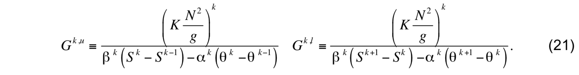
Due to the physical uncertainties surrounding the magnitude of the exchange coefficient K, considerable freedom exists in evaluating the term ∂ρ / ∂z in N2. One obvious choice was selected for use:

Having derived expressions for the vertical fluxes, the expressions used to advance layer thickness (mass flux), θ , and S in time will now be derived. Considering the mass flux first, the expression (d/ dt)(∂p / ∂ρ) is evaluated by converting (11) and (12) to flux form and integrating them across interfaces. This step is taken to remove the ambiguity that ∂θ / ∂t and ∂S / ∂t are indeterminate at interfaces. The flux equations for heat and salt, obtained in the usual manner by combining the advective forms of the equations with (13), are

and

Integrating these equations over an infinitesimally thin slab straddling layer interface k + 1 at the base of layer k (which will be denoted by k + 1 / 2 to avoid confusion with the layer index), the time tendency terms drop out because of the smallness of ∂p / ∂ρ, producing

and

By virtue of (20) and (21), the two previous expressions reduce to

This expression gives the mass flux at interface k + 1 / 2 which, in conjunction with the heat and salt fluxes given by (20), form a consistent set that can be used to solve the conservation equations for layer thickness, potential temperature, and salinity.
Inserting (26) into (13) and integration over layer k yields

The G terms have been grouped in a manner that mimics the second derivative of G with respect to k , which illustrates that diapycnal mixing tends to transfer mass from thick layers (N2 small) to thin layers (N2 large). The prognostic equations for heat and salt are obtained from the flux form of the conservation equations (22) and (23), which are integrated over the interior portion of layer k to produce

and

The G terms have again been arranged to highlight the diffusive nature of the equations. Equations (27) through (29) are integrated subject to the boundary conditions

When HYCOM is run with isopycnic coordinates (MICOM mode), the diapycnal mixing model from MICOM 2.8 is used. In MICOM 2.8, advection and diffusion in interior isopycnic layers are performed for salinity only, with layer temperature being diagnosed from the equation of state. The MICOM 2.8 interior diapycnal mixing algorithm is essentially model 2 above, but with only salinity and layer thickness being advanced in time and temperature diagnosed from the equation of state.
Large, W. G., J. C. McWilliams, and S. C. Doney, 1994: Oceanic vertical mixing: a review and a model with a nonlocal boundary layer parameterization. Rev. Geophys., 32, 363-403.
McDougall, T. J. and W. K. Dewar, 1998: Vertical mixing and cabbeling in layered models. J. Phys. Oceanogr., 28, 1458-1480.
Peters, H., M. C. Gregg, and J. M. Toole, 1988: On the parameterization of equatorial turbulence. J. Geophys. Res., 93, 1199-1218.