Every year the 32 NFL teams draft to select the next generation of NFL players. With the order going from worst to best record in the previous season, it's where teams try to ensure future success. What I wanted to analyze was if current methods used to value draft picks was optimal, and to see how important drafting is for team success.
According to Bill Belichick, all NFL teams use about the same valuation for draft picks, ESPN lists what is the consensus for the value of each pick. Under this valuation each pick is worth increasingly less than the previous pick. The valuation is used to make trades of draft picks; if you offer picks of equal or greater value it should be accepted.
When trying to find out a measure of player value that allowed for comparison across position I found a metric from Pro Football Focus called Approximate Value. The formula was created for just this purpose and uses a variety of statistics to determine the final product. The creator of Approximate Value, Doug Drinen, explained: "AV is not meant to be a be-all end-all metric. Football stat lines just do not come close to capturing all the contributions of a player the way they do in baseball and basketball. If one player is a 16 and another is a 14, we can't be very confident that the 16AV player actually had a better season than the 14AV player. But I am pretty confident that the collection of all players with 16AV played better, as an entire group, than the collection of all players with 14AV." For this project I used Weighted Average Value, as it values players with high peaks over those with consistent numbers over long careers. This helps account for injuries that derail promising careers, as well as that one exceptional season is much more likely to help win a super bowl, the ultimate goal of all NFL teams.
For this project I decided to use players drafted fro 2000 until 2022. The reason I used 2000 is not simply because of the new milenium, but because 2000 is the earliest draft class that had an active player in the 2022 season, Tom Brady. I combined all of the data from each draft class listed on Pro Football Reference into one spreadsheet, starting with Courtney Brown and ending with Brock Purdy.
In order to ensure the validity of the data I had to do a handful of tasks to ensure the data was accurate. The first was to add the year each player was drafted, allowing me to group each draft class. Next I had to make sure that the team each player was drafted by used the team’s current name. The Chargers, Rams, Raiders, and Commanders have all changed their official names, and other teams are listed under a different abbreviation, like the Packers being listed as GNB but are typically just called GB. Finally, I had to verify the accurate position of each player. Defensive players were not consistently listed for each position. Some players were not listed at Defensive End or Defensive Tackle, but rather just Defensive Line. Because very few were listed that way, I went and found the true position of every player listed at Defensive Line. For Linebackers, a small number were listed at Outside Linebacker or Inside Linebacker, but because the vast majority were just listed at Linebacker, I standardized all to just Linebacker. It was the same for Defensive Backs, almost all were listed at that position, so players listed at Safety or Cornerback were switched. Finally, Offensive Linemen without a specific position were also a very small number, so I found all of their true positions and switched them.
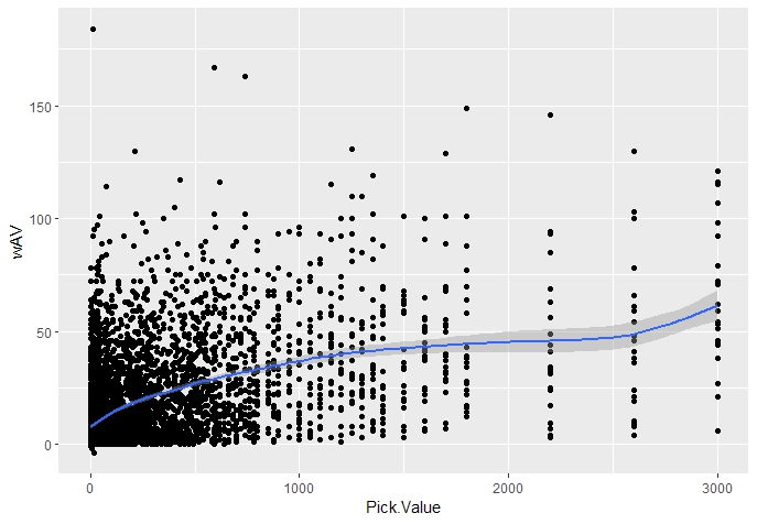
Because the space between picks is not constant, there is a large concentration of players with low value picks. However, the line drawn by R shows there is a increase in Weighted Approximate Value overall as Pick Value increases.
The first regression I created in R only used one variable, pick value, and it attempted to explain the Weighted Adjusted Value of players. The problem I encourted was the players drafted very recently were being compared against players who had played many more seasons and accumulated more Weighted Adjusted Value. Because I wanted an accurate representation of each player, I added year drafted as a second variable. The final regression I ended with was E[Weighted Approximate Value] = 9.50856+2.00706*(Pick Value^0.5)-8.71421*(2023-Year Drafted)^-0.3-1.97556*(Pick Value)^0.5*(2023-Year Drafted)^0.3.
I took the regression formula and plugged it into the original spreadsheet and compared the expected value to the the actual value and the top and bottom were no surprises. The greatest pick value was Tom Brady at pick 199 in 2000, followed by Drew Brees and Aaron Rodgers. The biggest bust was Charles Rodgers, whose career was derailed by injuries early on. Next after him is JaMarcus Russell and Jason Smith.
Next I created a pivot table based on the average difference between expected and observed Weighted Approximate Value. In the rows I put position and in the columns I put the round.
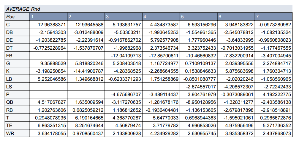 This table shows by round which positions have provided more wAV compared to the expected. For example, the best time to draft a Quarterback is the first round, with second round picks being the only others with a value greater than zero. Kickers and Punters generally perform better selected in the sixth or seventh rounds. Another interesting results is that Guards provide a positive value in every round, while defensive backs are always negative.
Using these values teams could maximize their value by targeting team needs based on how much value the pick is expected to provide. If they have a selection but all of their needs are negative or have higher returns later, the best decision would be to trade back.
A surprise I found was that as a whole, picks have a negative expected value. This means that overall that most of the picks made do not
This table shows by round which positions have provided more wAV compared to the expected. For example, the best time to draft a Quarterback is the first round, with second round picks being the only others with a value greater than zero. Kickers and Punters generally perform better selected in the sixth or seventh rounds. Another interesting results is that Guards provide a positive value in every round, while defensive backs are always negative.
Using these values teams could maximize their value by targeting team needs based on how much value the pick is expected to provide. If they have a selection but all of their needs are negative or have higher returns later, the best decision would be to trade back.
A surprise I found was that as a whole, picks have a negative expected value. This means that overall that most of the picks made do not
Back in R I used the NFLfastR package to visualize each team's success in drafting compared to how much was expected.
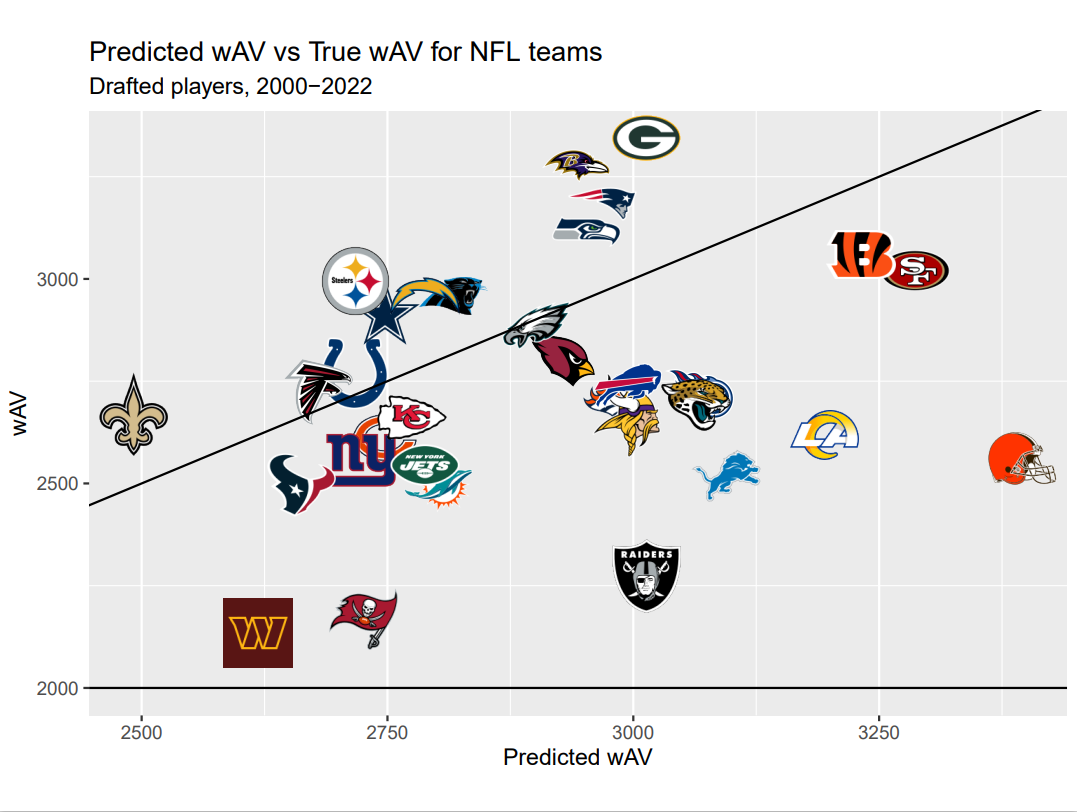 The line is y=x, meaning teams above the line got more value than was expected, while teams below got less. As expected, most teams do not properly utilize their picks based on traditional valuation, but 11 teams still over performed.
The last question I wanted to analyze was how important draft success was to team success. In R I made an additional plot with winning percentage on the Y axis and Observed wAV minus expected wAV with these results.
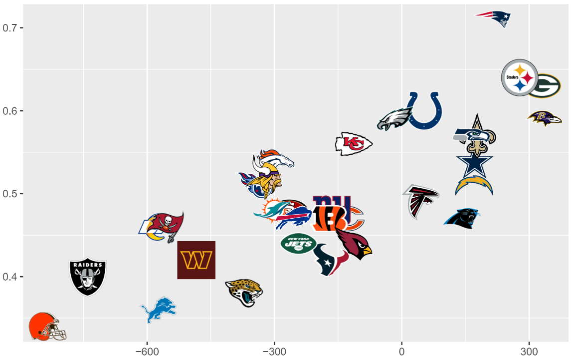 Looking at this graph it is obvious that there is a strong corelation; using draft value better leads to more games won.
Based on my analysis there is room for teams to improve their draft value analysis. The R-Squared provided by my regression provide more insight than the use of just traditional measurement. In addition to this, my model shows the track record for each position and round, and which positions are more likely for positive results. Finally, there is a clear positive correlation between performance in my metric and team winning percentage, the goal of NFL teams. If I were to do this again I would try to create a model that uses more than just two variables. Starting with position, but also things like NFL combine numbers, College stats, height, and weight to see what other ways player success can be predicted.