Facial Expression Prediction Using CNN - Group 4 - ECS 171 FQ 2022

Group Project for ECS 171, Fall Quarter 2022, at UC Davis under Dr. Solares.

Below is a link to our entire project notebook in Google Colab. We also have code blocks for certain sections located throughout this write-up

Group Members:

Member Name	GitHub Username
Alan Chuang	AlanChuang1
Daksh Jain	DakshJ4033
Sohum Goel	SohumGoel
Arnav Rastogi	Arnav33R
Grisha Bandodkar	grishaab

Introduction

• Our group stumbled upon the FER-2013 dataset as we were searching for ideas for the final project on Kaggle and other dataset websites. Since we enjoyed working with Neural Networks, we wanted to choose a dataset that allowed us to utilize convolutional layers to accurately classify information. We were excited to use it for our final project because it would give us an introduction to facial recognition on our phones and other applications.

• Having a model that accurately classifies images with certain emotions, features, age, race, etc is important as it can help improve facial recognition further and has many useful and applicable applications - such as, potentially catching/identifying criminals from an existing database.

• Thus, the aim of our project is to be able to predict the emotion that best fits a given facial expression. Although there is a plethora of possible emotions, our project focuses on a few that are the most basic human expressions/emotions. These are categorized as Angry, Fear, Happy, Neutral, Sad, Surprised, and Disgust.

Our Dataset

• This dataset contains images of faces that are 48x48 pixel grayscale and centered, thus occupying almost the same amount of space for each image, making recognition easier. Here are some examples of images contained in the dataset:

Methods

• Figure 1: Examples of images associated with the emotion fear

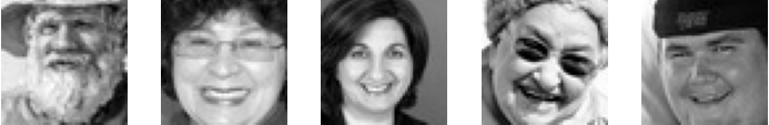
• Figure 2: Examples of images associated with the emotion happiness

Methods

How to Access Kaggle Datasets

• Please follow this tutorial to add kaggle dataset to google colab

• https://medium.com/unpackai/how-to-use-kaggle-datasets-in-google-colab-f9b2e4b5767c

Data Exploration

• There are 4,254 observations in the dataset, with 1774 happy observations, 1233 neutral observations, and 1247 sad observations. Each “observation”, or image file, is a 48x48 pixel-sized grayscale image of expressions on faces. Sizes are all standardized, so they don’t need to be cropped or require further changes.

• However, some images need to be flipped horizontally, and some need to be rescaled, which can be accomplished through Keras preprocessing (ImageDataGenerator). In order to normalize the images' pixels, we need to rescale the RGB coefficients to be in the range of 0 and 1.

Data Evaluation

• We create the dataframe by going through the directory and setting each image with its corresponding expression and storing that in a pandas dataset which is going to be returned by the function. We use the returned dataset to display the number of samples for each expression in our train and test dataset.

Data Evaluation

train_dir = './train/'
test_dir = './test/'

# image size
row, col = 48, 48
# number of image classes: angry, sad, etc
classes = 7

def count_exp(path, set_):
    dict_ = {}
    for expression in os.listdir(path):
        dir_ = path + expression
        dict_[expression] = len(os.listdir(dir_))
    df = pd.DataFrame(dict_, index=[set_])
    return df

# number of observations
train_count = count_exp(train_dir, 'train')
test_count = count_exp(test_dir, 'test')
print(train_count)
print(test_count)

• We then go through our directory again and plot an example image with the corresponding expression using our test data for the y-axis for simplicity.

test_count.transpose().plot(kind='bar',figsize=(12, 10))

plt.figure(figsize=(14,22))
i = 1
for expression in os.listdir(train_dir):
    img = load_img((train_dir + expression +'/'+ os.listdir(train_dir + expression)[1]))
    plt.subplot(1,7,i)
    plt.imshow(img)
    plt.title(expression)
    plt.axis('off')
    i += 1
plt.show()

Preprocessing

• Moving on, we preprocess our data by eliminating a class and reformatting the structure of all images. Next we remove disgust from the dataset. Then we create a single data frame consisting of all the images with their corresponding class (label).

shutil.rmtree( './train/disgust')
shutil.rmtree( './test/disgust')

# train dataset
images = []
labels = []
for subset in os.listdir(train_dir):
  image_list = os.listdir(os.path.join(train_dir,subset))  # all the names of images in the directory
  image_list = list(map(lambda x:os.path.join(subset,x),image_list))
  images.extend(image_list)
  labels.extend([subset]*len(image_list)) 

df = pd.DataFrame({"Images":images,"Labels":labels})      
df = df.sample(frac=1).reset_index(drop=True) # this will shuffle the data
samplesize = int(int(df.size)/14)  # sample size used for modelling 
print(samplesize)
df_train = df.head(samplesize)  

• Then, we used ImageDataGenerator() and flow_from_dataframe() via Keras preprocessing to go and apply various things such as rescale, color mode, size, class mode, shuffle, and subset filters to our training and validation subsets from the original dataframe. We will use these generators later in training and evaluating our model for accuracy. A similar process followed for the test data.

train_generator = datagen.flow_from_dataframe(
    directory = train_dir, 
    dataframe=df_train,
    x_col="Images",
    y_col="Labels",
    subset="training",
    batch_size=32,
    seed=42,
    shuffle=True,
    target_size=(48,48), 
    class_mode="categorical", 
    color_mode="grayscale"
)

Model 1

• In the first model we add two convolutional layers and 3 dense layers. Then its trained over 40 epochs. After that its complied using the Adam optimiser and categorical_crossentropy to compute loss.

• Model 1 was constructed with a simple CNN structure using a Keras Sequential model from TensorFlow, which groups layers of the model linearly and provides loss and accuracy values for our training and validation datasets.

• For our convolutional layer, we used Conv2D(), a layer to conduct spatial convolution over images to extract features from our images in the training dataset. For our pooling layer, we used MaxPooling2D() to downsample the input. We used Flatten() to prepare for the fully connected Dense layers, which are generated by Dense().

• The compile() method configures the model for training. The fit_generator() method accepts our training and validation generators and fits the model according to our sequential layers and returns validation and training loss and accuracy per epoch.

• We used the Adam() optimizer, which is a stochastic gradient descent method.

Model 2

• No new methods were introduced during this model, except more layers were added to the overall CNN.

Model 3

• We incorporated BatchNormalization() to normalize the inputs after each convolutional layer. We also used a Dropout() layer to prevent overfitting.

Model 4

• No new methods were introduced during this model, except more layers were added to the overall CNN.

Model 5

• In order to add penalties into the loss function that the CNN can optimize, we added layer weight regularizers to our convolutional layers.

Plotting Results

def plotValidationLossAccuracy(model):
    figure, axis = plt.subplots(1,2)
    figure.set_size_inches(16,6)

    train_ACC = model.history['accuracy']
    train_loss = model.history['loss']

    axis[0].plot(model.history['accuracy'], color = "green")
    axis[0].plot(model.history['val_accuracy'])
    axis[0].set_xlabel('Number of Epochs')
    axis[0].set_ylabel('Accuracy values')
    axis[0].set_title('Training against Validation Accuracy')
    axis[0].legend(['Train', 'Test'], loc = 'lower left')

    axis[1].plot(model.history['loss'], color = "green")
    axis[1].plot(model.history['val_loss'])
    axis[1].set_title('Training against Validation Loss')
    axis[1].set_xlabel('Number of Epochs')
    axis[1].set_ylabel('Loss Values')
    axis[1].set_title('Training against Validation Loss')
    axis[1].legend(['Train', 'Test'], loc ='lower left')

    plt.show()

• The ‘history’ object with .fit() stores all the training metrics for every epoch. Accuracy and Loss metrics are accessed after training by accessing the history object. Training and validation and comparing against each other for both of these metrics.

Retrieving Accuracy for a Model

def getAccuracy(model):
    train_loss, train_ACC = model.evaluate(train_generator)
    test_loss, test_ACC   = model.evaluate(valid_generator)
    print("The train accuracy = {:.3f} , test accuracy = {:.3f}".format(train_ACC*100, test_ACC*100))

• The function getAccuracy() evaluates the performance of the models. It prints out the final training and test accuracy obtained by the models.

Results

Data Evaluation

• This shows the number of samples for each expression in our train and test dataset.

• A bar chart that shows the total number of samples in each class along with an example image for each.

• Disgust class is removed from the dataset and will not be used in training the model. A single dataframe is created that holds all the images with their corresponding labels as shown in the below figure. Then all the images within are randomly shuffled and a sample is taken from it.

• All models ran for 40 epochs using the same training and validation generator from preprocessed data.

Model 1

• Model 1 generated a testing accuracy of 37.423%.

Model 2

• Model 2 generated a testing accuracy of 40.025%.

Model 3

• Model 3 generated a testing accuracy of 44.362%.

Model 4

• Model 4 generated a testing accuracy of 44.362%.

Model 5

• Model 5 generated a testing accuracy of 42.379%.

Code for working model:

model = tf.keras.models.Sequential()
# basic CNN

model.add(Conv2D(32, kernel_size=(3, 3), padding='same', activation='relu', input_shape=(IMAGE_SIZE, IMAGE_SIZE,1)))
model.add(MaxPooling2D(pool_size=(2, 2), padding="same"))

model.add(Conv2D(32, kernel_size=(3, 3), padding='same', activation='relu'))
model.add(MaxPooling2D(pool_size=(2, 2), padding="same"))

model.add(Flatten())

model.add(Dense(32, activation='relu'))
model.add(Dense(16, activation='sigmoid'))
model.add(Dense(6, activation='softmax'))

model.compile(
    optimizer = Adam(), 
    loss='categorical_crossentropy', 
    metrics=['accuracy']
  )

firstModel = model.fit_generator(generator=train_generator,
                    steps_per_epoch=STEP_SIZE_TRAIN,
                    validation_data=valid_generator,
                    validation_steps=STEP_SIZE_VALID,
                    epochs=40
)

Discussion

Data Exploration

• We selected this dataset because it contained ample photos of 7 different types of emotions, and it already separated the data into sorted directories. The sizes are all standardized and require little preprocessing.

• Using colored images would not be beneficial as grayscale is enough for classification, while color would add an extra dimension (r,g,b) and result in a complex and resource-intensive model.

• We also removed disgust from the dataset as it's small compared to the rest of the expressions, thus saving some time while training the model. We created a single data frame that stored all the images with their corresponding class (label). This made it easy for us to take a sample of the dataset because running the model on the entire dataset was extremely time-consuming.

• Flow_from_dataframe is specifically used because flow_from_directory is designed for datasets that have sub-directories (FER-2013) for each class, and we use a single data frame containing all the images.

Preprocessing

• Since all images were already the same size of 48x48 pixels, we did not further crop them. We decided to flip some images horizontally and rescale them. Normalization of the image pixels was important for classification, so the RGB coefficients were normalized to be within the range of 0 and 1. We chose grayscale images in order to ease classification.

• Ultimately, we could have added a shift for the width and height of the images in order to properly capture the face’s emotion for classification, or even add a zoom range. While running several iterations of models, we discovered that not only did it consume more time per epoch during training, but it also lowered validation accuracy significantly. Hence, we opted for a more simple preprocessed data set.

Model 1

• Model 1 had a barebones CNN structure: convolutional layers, pooling layers, and fully connected (dense) layers.

• The convolutional layers extract features from the image through a smaller kernel matrix over the image matrix. We decided to use 2 Conv2D layers, both with 32 filters to specify the depth of the feature map.

• After some research, we concluded that the most optimal kernel matrix size was (3,3). We added padding such that it adds zeros to become the size of the feature map. Relu was the best activation function for this context because it is generally used for each convolutional layer.

• Convolution layers and pooling layers are usually paired together. We used max pooling over average pooling in order to retrieve the maximum pixel value of each batch and focus on the brighter pixels. Generally, the pool size (2,2) was the most common in CNNs.

• We chose to add three dense layers with decreasing numbers of units. After playing around with different activation functions, we settled on relu, sigmoid, and softmax as the combination of the three performed better.

• We went with an Adam optimizer and a loss function of categorical cross-entropy which optimized accuracy.

• It is important to note that we used fit_genator() which is currently deprecated. For a future version, it should be replaced with fit(), passing the generators within the parameters.

• Reflecting on this model, it was very basic and performed adequately. The testing accuracy was low and the training accuracy was very high, which indicated the overfitting of the model.

Model 2

• Model 2 incorporated more layers in order to make the CNN more complex in hopes of better accuracy. After fitting the model and evaluating, it did perform better than Model 1.

• Overfitting is still a really big issue, since it shot up to 98% compared to the former 92%. This means that more layers actually contributed to the overfitting problem, but also improved testing accuracy.

Model 3

• In order to address the overfitting issue, we added batch normalization and dropout which should normalize the inputs and prepare them for the next layer.

• This model actually performed the best, it lowered the training accuracy (indicating the overfitting problem was slightly reduced) and improved the testing accuracy significantly.

Model 4

• Model 4 incorporated more layers in order to make the CNN more complex, while also increasing the number of times we use batch normalization and dropout.

• Overall, it didn’t necessarily improve the testing accuracy (in fact, it was exactly the same). It didn’t really help solve the overfitting problem, and the loss graph indicated a lot of uncertainty within the validation generator.

Model 5

• Regularizers help optimize the loss function in order to improve the testing accuracy, so we incorporated it in our layers.

• We also introduced a learning rate of 0.0001 in order to speed the training and improve optimization further. While it helped solve the overfitting problem, it did not necessarily improve the testing accuracy.

• In theory, this should have been our best model but this could be due to limitations in our training set or model.

Conclusion

• Model 3 performed the best with the highest testing accuracy of 44.362% and the least relative overfitting. If we had more computing power, we would have run the model on the entire dataset which might further improve the testing accuracy.

• Since the dataset was huge, it was not feasible for us to do that. We also could have used more complex preprocessing, but that caused a lot of issues since it significantly increased training time per epoch in every model.

Extended application:

• Training the model on more intricate expressions could make the model more sensitive to subtle facial expressions. This project could be applied in real time to analyze expressions in crowded areas, such as bars, to prevent crimes.

• There are also social applications for such a project, such as AI interactions with humans. If we could accurately predict human expressions and emotions using computer vision, we could create virtual therapists that can correctly analyze facial expressions. There could also be further implementations of this in neurotech and machine learning. In fact, this already exists today, in the form of algorithms that analyze the level of motivation for stroke patients undergoing therapy.

Collaboration

• Alan Chuang: I worked on composing parts of the writeup as well as organizing the final format presentation, and also did some initial debugging. We all worked towards setting up meetings and meeting deadlines, and contributed equally to complete this project, which was a great learning opportunity!

• Daksh Jain: I was responsible partially for coding, debugging, and communicating with team members to set up meetings and manage deadlines. I also worked on the write up introduction and Methods section. We split tasks evenly and helped each other when needed. I believe everyone in the group worked hard and together as a team!

• Sohum Goel: I was responsible for the initial setup of the neural network, along with some trial runs. I also contributed towards the write up. We added to each other's work. Everyone worked together to complete this project.

• Grisha Bandodkar: I mainly worked on training and running multiple iterations of the model such that it could get the best possible accuracy results. I contributed towards the results, discussion, and conclusion sections of the write up. Everyone contributed equally toward this project.

• Arnav Rastogi: I worked largely on the write-up, but also partially on debugging and organizing the repository, along with coordinating with team members to manage milestone deadlines and fix meeting times. We all contributed equally, coordinated well, and worked together on this project

Appendix/Sources

[1]R. Pramoditha, “Coding a Convolutional Neural Network (CNN) Using Keras Sequential API,” Medium, Jun. 28, 2022. https://towardsdatascience.com/coding-a-convolutional-neural-network-cnn-using-keras-sequential-api-ec5211126875

[2]Darshil, “How to create effective CNN for your use-case,” Analytics Vidhya, Jul. 18, 2021. https://medium.com/analytics-vidhya/how-to-create-effective-cnn-for-your-use-case-6bae5c6871f6 (accessed Dec. 08, 2022).

[3]R. Gandhi, “Build Your Own Convolution Neural Network in 5 mins,” Medium, May 18, 2018. https://towardsdatascience.com/build-your-own-convolution-neural-network-in-5-mins-4217c2cf964f (accessed Dec. 08, 2022).

[4]A. Jayasankha, “Build your own model with Convolutional Neural Networks,” Analytics Vidhya, Aug. 28, 2020. https://medium.com/analytics-vidhya/build-your-own-model-with-convolutional-neural-networks-5ca0dd222c8f (accessed Dec. 08, 2022).

[5]R. Prabhu, “Understanding of Convolutional Neural Network (CNN) — Deep Learning,” Medium, Mar. 04, 2018. https://medium.com/@RaghavPrabhu/understanding-of-convolutional-neural-network-cnn-deep-learning-99760835f148

[6]Y. Fan et al., “FER-PCVT: Facial Expression Recognition with Patch-Convolutional Vision Transformer for Stroke Patients,” Brain Sciences, vol. 12, no. 12, p. 1626, Dec. 2022, doi: 10.3390/brainsci12121626.