EigsysClustering

EigsysClustering is an open-source Python toolkit for unsupervised identification of topological phases of matter using an Eigensystem vector representation combined with Gaussian Mixture Model (GMM) clustering. It implements the method from Precise Identification of Topological Phase Transitions with Eigensystem-Based Clustering and enables researchers to easily apply this approach to their own quantum models. The method requires minimal feature engineering and no prior labels, yet achieves high accuracy in detecting phase transitions.

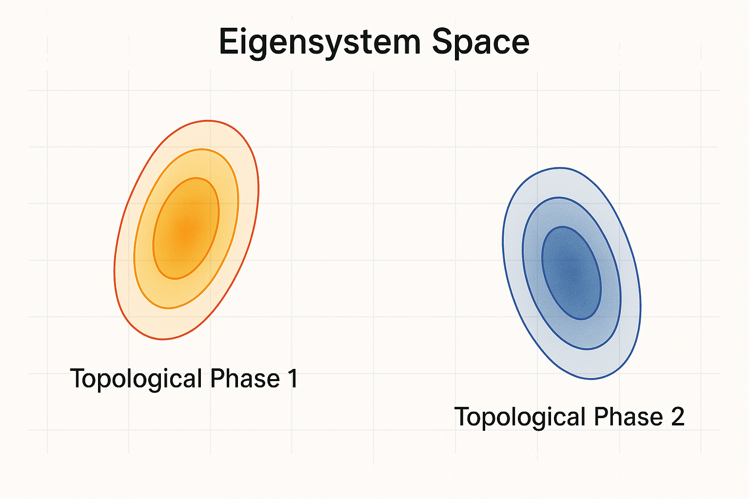
Figure 1: Eigensystem vector representation of Hamiltonians forms well-separated Gaussian clusters corresponding to distinct phases.

Introduction

Topological phases exceeds traditional Landau-Ginzburg paradigms, and their classification is a central problem in modern condensed matter physics. Existing ML approaches often relied on supervised learning with carefully chosen physical features, or unsupervised learning by Diffusion Map Embedding + KMeans Clustering.

EigsysClustering provides a simple yet effective unsupervised alternative: represent each Hamiltonian by its full set of eigenvalues and eigenvectors, sorted and gauge-fixed in certain way, forming an eigensystem vector, and cluster these vectors using a GMM.

This enables automatic discovery of phase boundaries with little domain knowledge, and achieves higher accuracy in our studied scenarios than current state-of-the-art diffusion map method.

Moreover, this method reveals an interesting physics insight that distinct topological phases are Gaussian-distributed clusters in the high-dimensional eigensystem space.

Key features of the Eigensystem-based approach:

• Unsupervised phase classification: Distinct topological phases are identified with near 100% accuracy without any prior labels.
• Precise phase boundaries: Phase transition points are pinpointed with high resolution (on the order of O(10⁻⁵) in parameter space for studied examples).
• Minimal tuning: No complex feature engineering or hyperparameter tuning is required – the eigensystem is a direct representation.
• Scalability: A simple linear dimension reduction (e.g. PCA) can be applied to eigensystem vectors to reduce dimensionality from O(N²) to O(N) with negligible loss in accuracy.
• Generality: Successful on multiple 1D models (Hubbard Spin-Orbit Coupled Fermi chain, Kitaev chain, Su–Schrieffer–Heeger model, non-Hermitian SSH model), reliably clustering phases across different systems.

Installation

Some core computations of EigsysClustering use PyTorch (for a baseline method, diffusion map clustering) and TensorFlow (optional, for faster batched eigen-decompositions) and, so both frameworks should be installed. One can either refer to the official installation instructions for TensorFlow and PyTorch to set up the environment as per your machine's specifications and OS; or, preferably, create a new conda environment.

1. Create a conda environment (recommended):

$ conda create -n eigsys python numpy sympy pandas pytorch -c conda-forge -c pytorch
# Optional: `$ conda install tensorflow`
$ conda activate eigsys

(Alternatively, ensure tensorflow and torch are installed in your environment.)

2. Clone the repository and install the package:

$ git clone https://github.com/sarinstein-yan/EigsysClustering.git
$ cd EigsysClustering
$ pip install .

3. Verify the installation:

import eigsys as es
print(es.__version__)

Optionally, install giotto-tda for Topological Data Analysis (TDA) by $ pip install giotto-tda.

Example Usage

Below we demonstrate the usage of EigsysClustering on a well-known 1D topological model -- the Kitaev chain (1D p-wave superconductor). We will define the model's Hamiltonian symbolically, sample a range of parameters to generate a dataset of Hamiltonians, construct the eigensystem vectors, and then apply clustering to discover the topological phase transition. Finally, we’ll evaluate clustering performance and test noise robustness. The same workflow can be applied to other models by defining the appropriate Hamiltonian.

Defining the Hamiltonian

We use SymPy to define the Bloch Hamiltonian (i.e. Hamiltonian in momentum space) matrices symbolically. For convenience, we first define Pauli matrices and then the Bloch Hamiltonians for some one-dimensional, two-band models:

import sympy as sp

# Define Pauli matrices
pauli_x = sp.ImmutableMatrix([[0, 1], [1, 0]])
pauli_y = sp.ImmutableMatrix([[0, -sp.I], [sp.I, 0]])
pauli_z = sp.ImmutableMatrix([[1, 0], [0, -1]])

# Momentum symbol
k = sp.symbols('k', real=True)

# Define Bloch Hamiltonians for different models:
def h_Kitaev(k, mu, t=1, Delta=0.3):
    # 1D Kitaev p-wave superconductor (p-wave pairing Delta)
    return -(mu + 2*t*sp.cos(k))*pauli_z + 2*Delta*sp.sin(k)*pauli_y

def h_HubbardSOC(k, m_z, t_s=1, t_so=0.3):
    # 1D Fermi chain with spin-orbit coupling (SOC) and Zeeman field m_z
    return (m_z - 2*t_s*sp.cos(k))*pauli_z - 2*t_so*sp.sin(k)*pauli_x

def h_SSH(k, v, w=1, s=0):
    # Su-Schrieffer–Heeger (SSH) chain; `s` introduces non-Hermitian perturbation `s i sigma_y` if nonzero
    h = (v + w*sp.cos(k))*pauli_x + w*sp.sin(k)*pauli_y
    if s != 0: h += s*sp.I*pauli_y
    return h

In this example, we will focus on the Kitaev chain. Its Bloch Hamiltonian h_Kitaev(k, μ) is defined above. The model has a topological phase for chemical potential μ < 2t and a trivial phase for μ > 2t when the pairing term Δ is nonzero.

Sampling Hamiltonians across parameter range

We next generate a dataset of Hamiltonians in both phases by sampling in the parameter space (i.e. the μ axis). For the Kitaev model, we scan μ from 0 to 4 (covering both phases) for a chain of length N=10. The helper function es.H_1D_batch parallelly constructs an array of desired real-space Hamiltonian (both under open and periodic boundary conditions) for arrays of input parameter values.

import numpy as np
import eigsys as es

# Define the Kitaev Bloch Hamiltonian symbolic expression
mu = sp.symbols(r'\mu', real=True)
h_k = h_Kitaev(k, mu=mu, t=1, Delta=0.3)
# Sample parameter μ over a range
mu_values = np.linspace(0, 4, 1000)
# chain length (number of sites)
N = 10
# ^ small sample size and system size for ease of demonstration

# Generate real-space Hamiltonian matrices for each μ value
H_obc, H_pbc = es.H_1D_batch(h_k=h_k, k=k, N=N, param_dict={mu: mu_values})

print("Hamiltonian samples array shape (PBC):", H_pbc.shape)
---
>>> Hamiltonian samples array shape: (1000, 40, 40)

Here H_pbc is a NumPy array of shape (1000, N*d, N*d) where d=2 is the degree of freedom per unit cell (spin), equivalent to the number of energy bands.

We will use the periodic-boundary version H_pbc for eigendecomposition to obtain the eigensystem vectors. The open-boundary version H_obc is used instead for non-Hermitian models (e.g. SSH with nonzero s) due to non-Hermitian skin effect (NHSE).

We also prepare the "ground truth" phase labels for evaluation (not needed for clustering itself, but useful to calculate accuracy later):

# True phase labels for each sample (1 = topological, 0 = trivial)
y = np.where(mu_values < 2*1, 1, 0)

In the above Kitaev model, the critical point is at μ = 2t = 2, so μ < 2 is topological (winding number = 1) and μ > 2 is trivial (winding number 0).

Constructing eigensystem vectors

Now, we diagonalize all Hamiltonians in one shot. EigsysClustering prioritizes the use of TensorFlow's vectorized, high-performance eigen-solver and wraps in es.eig_batch to diagonalize a large batch of matrices more efficiently.

es.eig_batch can be optionally accelerated on GPU by passing a device string in either tensorflow or torch format (assuming at least one of them can be imported, otherwise the device string will be ignored and fallback to numpy).

We then obtain the eigensystem vectors with es.eigsys_vecs:

import tensorflow as tf, torch, os
os.environ['TF_GPU_ALLOCATOR'] = 'cuda_malloc_async'  # (optional, for TensorFlow GPU memory optimization)

# Diagonalization
eig_vals, eig_vecs = es.eig_batch(
    H_pbc, 
    device='/GPU:0', 
    # ^ Provided a GPU is available, the default `device` is `/CPU:0`.
    is_hermitian=True, 
    chop=False, 
    # ^ If true, chop small values for numerical stability
)

# Construct "eigensystem vectors" for all samples
X = es.eigsys_vecs(eig_vals, eig_vecs)
print("Eigensystem feature matrix shape:", X.shape)
---
>>> Eigensystem feature matrix shape: (1000, 420)

At this point, X is a NumPy array of shape (1000, M) where M = N×d (N×d + 1) = 420 for N=10. This is our feature dataset (design matrix) in eigensystem space.

For insight into the dataset structure, we can compute the pairwise distance matrix or a kernel (similarity) matrix:

# Compute pairwise Euclidean distance matrix and Gaussian (RBF) kernel matrix
dist_matrix = es.distance_matrix(X, metric='euclidean')
kernel_matrix = es.kernel_matrix(X, metric='rbf')

The distance matrix (dist_matrix) is 1000×1000 where entry (i,j) is the Euclidean distance between sample i and j in eigensystem space; the Gaussian (RBF) kernel (kernel_matrix) measures similarity (with entries closer to 1 for similar Hamiltonians). If our data naturally clusters into two phases, we expect to see a block structure (small intra-cluster distances, larger inter-cluster distances).

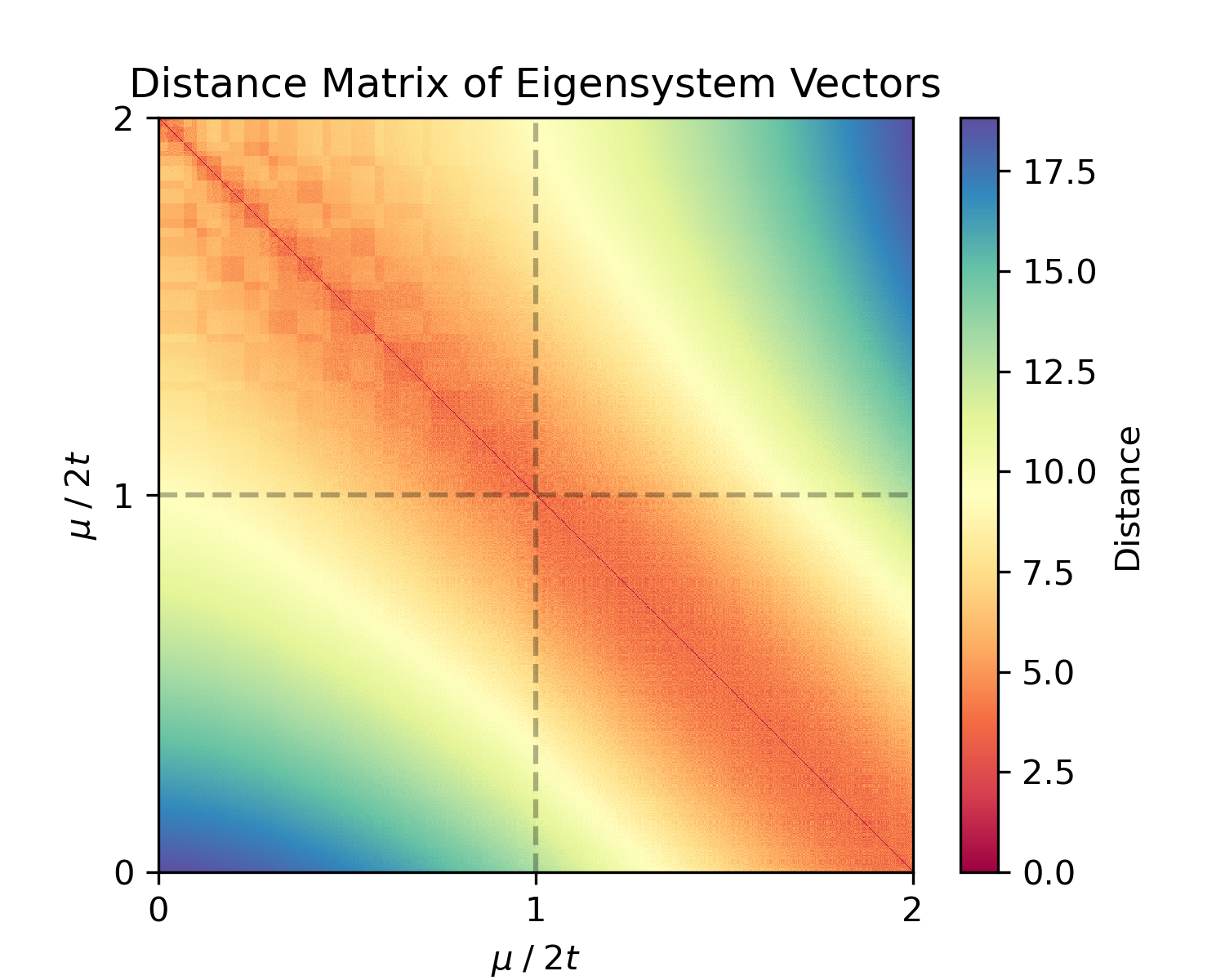
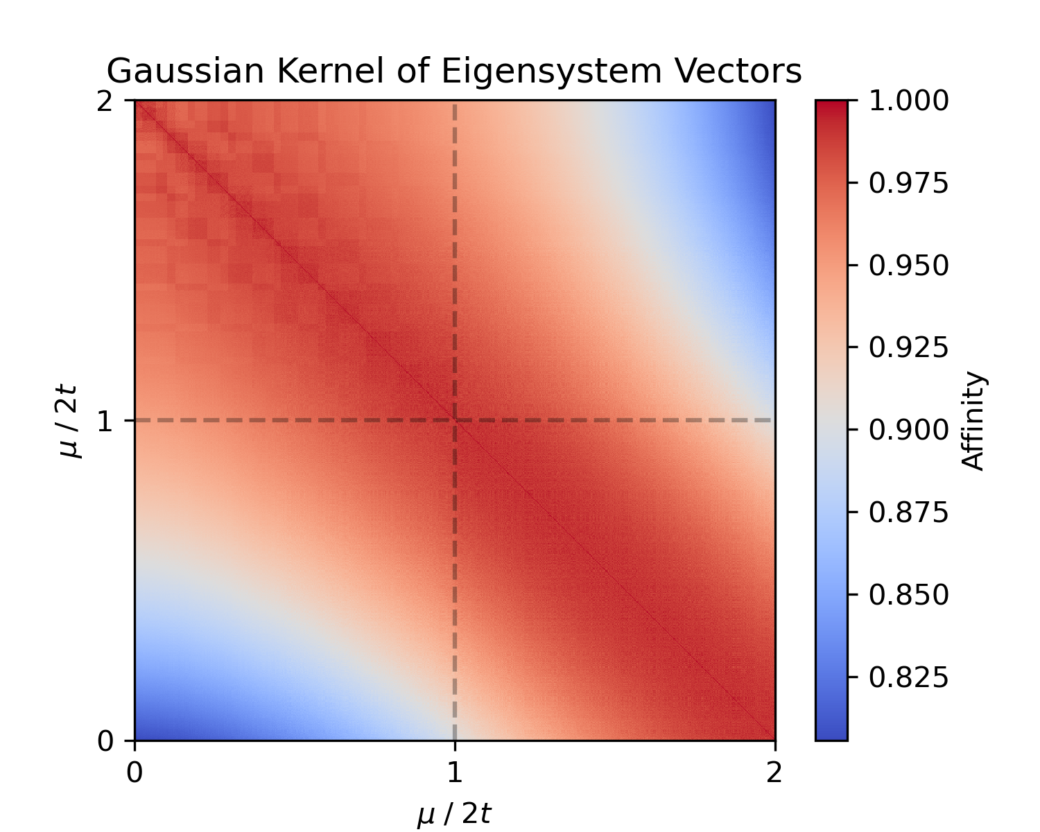
Figure 2: Euclidean Distance matrix and Gaussian kernel similarity matrix for the eigensystem vectors of the sampled Hamiltonians.

Clustering and evaluation

With the eigensystem vector dataset X ready, we can apply clustering algorithms to separate the topological vs trivial phases. EigsysClustering provides a convenient ClusteringEvaluator class in scikit-learn style that can run multiple clustering methods and evaluate them against the known labels. We will use GMM (Gaussian Mixture Model), KMeans, Spectral Clustering, and Diffusion Map for comparison:

# Initialize the clustering evaluator for 2 clusters (phases)
evaluator = es.ClusteringEvaluator(
    n_clusters=2, random_state=0,
    methods=('gmm', 'kmeans', 'spectral', 'dmp'),
    diffusion_time=1, epsilon=10 # < hyperparameters for diffusion map clustering
)
# Fit all specified clustering methods on the data X
evaluator.fit(X, y)

# Retrieve results as a pandas DataFrame
results_df = evaluator.result_df

The methods tuple specifies which clustering approaches to run:

• 'gmm': Gaussian Mixture Model clustering.
• 'kmeans': K-Means clustering.
• 'spectral': Spectral clustering (Laplacian-based), using Nearest Neighbor kernel.
• 'dmp': Diffusion Map Embedding + KMeans clustering (as per Rodriguez-Nieva et al. 2019, implemented internally via DiffusionMapTorch for embedding only and DiffusionClustering for whole pipeline).

After calling fit, evaluator.result_df contains metrics for each method: e.g. Accuracy, Adjusted Rand Index (ARI), Adjusted Mutual Info (AMI), Calinski-Harabasz score, Davies-Bouldin index, and Silhouette coefficient.

One can convert the row-wise dataframe to spreadsheet style for better readability:

evaluator.as_spreadsheet() # or `evaluator.to_wideform()`

This line should give a similar output as the following:

Method	AMI	ARI	Accuracy	CalinskiHarabasz	DaviesBouldin	Silhouette
GaussianMixture	1.000	1.000	1.000	1417.65	0.812	0.471
DiffusionMap	0.785	0.835	0.957	1449.48	0.799	0.473
KMeans	0.754	0.803	0.948	1450.04	0.796	0.473
SpectralClustering	0.496	0.470	0.157	317.95	1.421	0.225

(Above, ARI/AMI = 1 indicates perfect clustering matching true labels.)

For this example, one should observe that GMM perfectly clusters the two phases, whereas other methods perform worse (even with a bit of hyperparameter tuning).

Noise robustness test

One important validation is how robust the clustering is to noise in the data. We can simulate experimental noise by adding random perturbations to the eigensystem vectors and see if the phase classification still holds. The ClusteringEvaluator.noise_robustness_test automates this by adding Gaussian noise and evaluate performances over several trials:

evaluator.noise_robustness_test(noise_levels=[0.5, 1.0, 2.0, 3.0], method='gmm', n_iter=10)
noise_test_df = evaluator.noise_test_result

# Show the mean and std of different metrics
noise_test_df.groupby('Noise Level').agg(['mean', 'std'])

In the above, we test noise with standard deviation 0.5σ, 1σ, 2σ, 3σ (where σ is the standard deviation of each feature in the original data) and run 10 random trials for each. The results of all runs are stored in evaluator.noise_test_result.

The last line aggregates the results by noise level, showing the mean and standard deviation of each metric at each noise level. You should get a result similar to:

Noise Level	Accuracy	ARI	AMI
0.5	0.956 ± 0.008	0.833 ± 0.030	0.783 ± 0.030
1.0	0.939 ± 0.005	0.770 ± 0.019	0.706 ± 0.022
2.0	0.892 ± 0.005	0.615 ± 0.017	0.517 ± 0.019
3.0	0.833 ± 0.011	0.444 ± 0.030	0.351 ± 0.026

We observe that GMM shows good resilience to noise. For example, the clustering accuracy only drops to ~96% at 0.5σ noise and ~83% at 3σ noise.

Concluding Remarks

EigsysClustering provides a set of high-performance, easy-to-use tools for unsupervised clustering of topological phases. By following the above example, users can adapt the workflow to other Hamiltonian models: simply write down your own Bloch Hamiltonian and EigsysClustering will handle the rest.

This package is optimized for speed and efficiency, contains multiple built-in clustering backends and supports custom clustering methods, facilitating exploration of large parameter spaces.

We hope this package accelerates research into phase discovery and invites further extensions, such as "rebuild the quantum mechanics" starting from the eigensystem space -- the eigensystem vector contains all relevant information about the Hamiltonian, and obviously the dominant global structure of the eigensystem space is the topological phase structure.

One may expect that the substructure of the eigensystem space (e.g. local minima, saddle points) may also contain physics relevant information about the Hamiltonian.

Happy clustering!